Assignment 2: Lambda Theory

Due: Thursday, October 10 at 11:59pm
Submission cutoff: Saturday, October 12 at 11:59pm

This week, we looked at the theory behind the untyped and simply-typed lambda calculi. In this assignment, you will do a deep dive into the computational power of the untyped lambda calculus. Rather than just considering language-level rules, you will write actual lambda calculus programs to perform numeric operations. You will also work through a few different changes and extensions to the lambda calculi.

Setup

In the f19-assignments repository, run git pull to get the assignment materials, located in the assign2 directory.

1: Church encoding (30%)

Part of understanding a computational model is knowing its expressiveness: what range of programs can be written in the model? For example, in the language of arithmetic, we know that every program must evaluate to a value, i.e. it can never loop. While most normal programming languages permit partial functions (functions that could return a result or loop forever), we’ve proven that arithmetic is a language of total functions (they always return a result).

Intuitively, this means that arithmetic is less expressive than more general programming languages. The set of programs expressible in arithmetic is a strict subset of those expressible in, say, Python or Java. What about the lambda calculus? It seems like such a simple language, but can we formally reason about its expressiveness? It turns out the lambda calculus is equivalent in expressiveness to a Turing machine—this result is called the Church-Turing thesis. Both of these computational models can express computable functions. Informally, a computable function is “a function on the natural numbers computable by a human being following an algorithm, ignoring resource limitations.”

In the context of the lambda calculus, this idea will seem strange. If we only have variables and functions, how are supposed to express something as simple as ($2+2$)? The key idea is that we have to provide a mapping from constructs in the lambda calculus to natural numbers, which allows us to interpret the result of a lambda calculus program as a number. This is called the Church encoding. In the remainder of this section, we’ll work through a few exercises to understand how this encoding works.

1.1: Numbers (10%)

First, we’ll look at how to interpret a lambda calculus program as a natural number. This construction derives from Peano numerals, which is essentially the “tally marks” approach to representing numbers that we discussed in the first lecture. Here, ($Z$) is the number ($0$), and $S(n)$ is the number ($n + 1$). For example:

• ($Z = 0$)
• ($S(S(Z)) = 2$)
• ($S(S(S(S(S(Z))))) = 5$)

A Church numeral for ($n$) is a lambda calculus function that takes two arguments ($f$) and ($x$), and applies ($f$) to ($x$) a total of ($n$) times. For example:

• ($\fun{f}{\fun{x}{x}} = Z = 0$)
• ($\fun{f}{\fun{x}{\app{f}{(\app{f}{x})}}} = S(S(Z)) = 2$)
• ($\fun{f}{\fun{x}{\app{f}{(\app{f}{(\app{f}{(\app{f}{(\app{f}{x})})})})}}} = S(S(S(S(S(Z))))) = 5$)

Key idea: a function can be a number, and what’s in the function defines exactly what number. It’s all a matter of interpretation.

We can then define lambda calculus functions to emulate functions on numbers. For example, the successor operation adds one to the input number ($n$):

Why does this work? Let’s walk through an example. If we evaluated ($S(2)$), this would look like:

If this expression was the church numeral for 3, then it would apply the function ($f$) to ($x$) three times. Is that the case? Even though it’s not technically part of the semantics, we can simplify inside parts of the number to answer this question.

From this, we can see that the resultant function does apply ($f$) three times to ($x$), hence this is the church numeral for three, and our successor function appears to work.

Now let’s mechanize this. In the assign2/program directory, we have provided a binary lci_{platform}, or lambda calculus interpreter, that executes an lambda calculus program and interprets it as a church numeral. Try this out:

$ ./lci_macos
> fun f -> fun x -> x
0
> z = fun f -> fun x -> x
> s = fun n -> fun f -> fun x -> f (n f x)
> (s (s z))
2

Note: this is a slightly modified version of the lambda calculus with persistent identifiers.

You can also use the interpreter to execute a standalone file.

$ cat test.lam
z = fun f -> fun x -> x
s = fun n -> fun f -> fun x -> f (n f x)
(s (s z))

$ ./lci_macos test.lam
Expression on line 3 evaluated to 2

Your first task is to define a multiply function. As per the Church encoding Wiki page, the addition and multiplication functions are usually defined as follows:

Instead of this definition, your job is to provide an alternate implementation of ($\msf{mult}$) that only uses ($\{m, n, \msf{plus}, Z\}$), as well as parentheses. A few hints.

1. Fill in the template: ($\msf{mult} = \fun{m}{\fun{n}{\underline{\hspace{3cm}}}}$)

2. Remember that although ($m$) and ($n$) represent numbers, they are still functions that you can use however you like.

3. Use the interpreter to help you experiment!

4. A key idea here is partial evaluation. In this style of programming, if you give a function less than the expected number of arguments, it returns a function that waits on the remaining ones. For example, $\mathsf{plustwo} = \mathsf{plus}\ 2$ is a function that adds 2 to a number, e.g. $\mathsf{plustwo}\ 3 = 5$.

Put your answer in the assign2/program/mult.lam file.

1.2: Booleans (10%)

To introduce conditional logic, i.e. ifs/thens/comparisons, we need to use the Church encoding for booleans. Here, the idea is that true and false are functions which select a particular branch of two possibilities.

For example, $\app{\app{\msf{true}}{Z}}{(\app{S}{Z})} \mapsto Z$. From this, we can define our essential conditional operators:

Again, see the Wiki page for more explanation and examples. In this section, your challenge is to define a function ($\msf{even}$) that takes as input a number, and returns true if it’s even, and false otherwise. You can only use the input number and the ($\{\msf{true}, \msf{false}, \msf{not}, \msf{if}\}$) constructs (no recursion!). Some hints:

1. Fill in the template: ($\msf{even} = \fun{n}{\underline{\hspace{3cm}}}$)

2. We can inductively define the $\msf{even}$ function over the natural numbers as: ($\app{\msf{even}}{Z} = \msf{true} \mid \app{\msf{even}}{S(n)} = \app{\msf{not}}{(\app{\msf{even}}{n})}$)

Put your answer in the assign2/program/even.lam file.

1.3: Recursion (10%)

A last critical piece missing from our computational framework is the idea of recursion. In the basic formulation given, you can’t trivially recurse within a function. When declaring a function, you can’t get access to the identifier binding the function. For example, when defining a recursive sum in Javascript, we can usually write:

function sum(n) {
  if (n == 0) { return 0; }
  else { return sum(n - 1) + n; }
}

Where we are allowed to reference sum inside of its own definition. But in the lambda calculus, if we try this idea:

Here, $\msf{iszero}$ returns true if the input is zero and false otherwise. $\msf{pred}~n$ returns $n - 1$.

Then this is an invalid expression, because $\msf{sum}$ isn’t bound in the function. Instead, we can use the amazing magics of the fixpoint combinator (or more famously, the “Y combinator”). The fixpoint combinator looks like this:

The $\msf{fix}$ function has the curious property of a fixpoint, which is that $\app{\msf{fix}}{f} = \app{f}{(\app{\msf{fix}}{f})}$ for all $f$. See an extended example of this on the Wiki page.

Intuitively, the way we can use the fixpoint combinator is to provide a function with a handle to itself—this is the idea of self-reference. For example, we can define an infinite sum:

More practically, we can define recursive functions that terminate using conditions like in the Javascript example above. Your challenge in this section is to use the fix combinator to create a recursive sum function that adds the numbers from 1 to $n$. You can use any of the constructs defined in the above sections or on the linked Wikipedia pages (except don’t use the closed form!).

Put your answer in assign2/program/sum.lam.

If you wanted to, how would you complete the proof of the equivalence of the lambda calculus and Turing machines? Once you have numbers, booleans, and a fixpoint, it’s only a short jump to simulating a Turing machine inside the lambda calculus. You would need a notion of lists and tuples (and a way of getting input), and then you can define a function:

step : (number /*state*/, list /*tape*/) -> number /*input*/ -> (number /*state*/, list /*tape*/)
s0 = pair 0 empty
tm = fix (fun tm -> fun s -> tm (step s (get_input ())))

Out of respect for your time, I’ll leave this as an optional exercise for the reader.

2: Dynamic scoping (30%)

Credit to Stephan Boyer for the inspiration.

Lexical vs. dynamic scoping

Recall from class that scope is the central idea in programming languages of: given a variable, what binding does it refer to? For example, consider this program (in Javascript):

let x = 1;
function g(z) { return x + z; }
function f(y) {
  let x = y + 1;
  return g(y * x);
}
console.log(f(3));

When executing the inner g function, it has the following call stack:

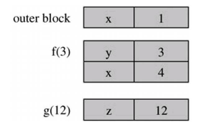
Take a second to walk through the code and verify this diagram matches your expectations. When executing g, the name resolution question here is: in the expression x + z what does x refer to? There are two options: the x defined in the top-level scope, and the x defined in the function f.

The first option, picking x = 1, is called lexical scoping. The intuition behind lexical scoping is that the program structure defines a series of “scopes” that we can infer just by reading the program, without actually running the code.

// The {N, ...} syntax indicates which stack of scopes are "active" a given
// point in the program.

// BEGIN SCOPE 1 -- {1}
let x = 1;
function g(z) {
    // BEGIN SCOPE 2 -- {1, 2}
    return x + z;
    // END SCOPE 2
}
function f(y) {
  // BEGIN SCOPE -- {1, 3}
  let x = y + 1;
  return g(y * x);
  // END SCOPE
}
console.log(f(3));
// END SCOPE 1

The nested structure of our program implies that at any line, we have a stack of scopes as annotated in the program above. To resolve a name, we walk the stack and search for the closest declaration of our desired variable. In the example, because scope 3 is not in the stack of scope 2, x + z resolves to the binding of x in scope 1, not scope 3.

Again, we call this “lexical” scoping because the scope stack is determined statically from the program source code (i.e. before the program is executed). The alternative approach, the one that resolves to x = 4, is called dynamic scoping. Recall our call stack above:

As you may have inferred at this point, dynamic scoping looks at the runtime call stack to find the most recent declaration of x and uses that value. Here, the binding x = 4 in f is more recent than the binding x = 1 in the top-level scope.

In both cases, dynamic or lexical, the core algorithm is the same: given a stack of scopes, walk up the stack to find the most recent name declaration. The only difference is whether the the scope stack is determined before or during the program’s execution.

Scoping in the lambda calculus

Let’s now contextualize these ideas in the lambda calculus. The classical presentation of the lambda calculus is always lexically scoped, i.e. a variable always refers to the closest lambda with the same argument variable in the syntax tree. However, it’s possible to tweak the evaluation rules and implement dynamic scoping in the lambda calculus. For example, consider the expression:

Conventions: as a shorthand, we’re using the underscore for a variable that doesn’t matter, and the asterisk for a value whose specific value does not matter (it could be anything and the example does not change). $L$ and $D$ are both values.

Under normal lexical scoping rules, this evaluates to:

However, under a dynamic scoping system, the exact same example would evaluate to a different answer. Here’s the trace under such a scoping system:

This execution trace should look strange to you. We’re evaluating the inside of a function without substituting the variable! Let’s look at the operational semantics to better understand this idea.

Whereas in lecture we used a proof context in the typing rules, here we use a proof context for our operational semantics. The proof context is a set of variable mappings, similar to our runtime stack in the Javascript example. The syntax $\ctx, x \rightarrow e_2$ means “add $x \rightarrow e_2$ to the context $\ctx$”. Like a normal dictionary, a new mapping can overwrite a previous one, for example:

The crux of the construction is in the D-App-Body rule. To evaluate a function, we step the body $e_1$ while placing $x \rightarrow e_2$ into the proof context. This allows any expression within $e_1$ to use $x$, even if it wasn’t in its lexical scope. Leaving $e_2$ in the syntax while we step the function body is essentially using the syntax to maintain a runtime stack, which we reconstruct in our proof context on every small step.

For another clarifying example, here’s a valid expression:

Even though the $x$ is not in the lexical scope of the function $f$, this will still evaluate to $D$ because $x$ is bound while $f$ is being executed.

Stop. Re-read the above two sections and ensure that you understand what dynamic scoping means, and why these semantics implement it. Most of your time in this part of the assignment will likely be spent understanding the background, not performing the task.

2.1: Evaluation proof (15%)

Using the above semantics, we can produce a formal proof to justify each step in the provided example trace. Below, we have provided you with the first step in the proof—your task is to fill in the proof for the remaining three steps.

Put your answer in part 2 of the written solution.

2.2: New semantics (15%)

Your final challenge is to extend the dynamically scoped lambda calculus with a new construct, the let statement. Let statements are like functions in that they bind variables for use in an expression. For example:

We could rewrite the initial example as:

More generally, we extend our grammar with the following construct:

Provide the operational semantics for the let statement that preserves dynamic scoping. The reference solution contains two inference rules. Put your answer in part 2 of the written solution.

3: Typed language extensions (40%)

Eager to gain the approval of the functional programming community, Will has submitted two potential extensions to the simply-typed lambda calculus. For each extension, he wrote down the proposed statics and dynamics. Unfortunately, his eagerness led him astray, and only one of these extensions is type safe—the other violates at least one of progress and preservation.

Your task is to identify which extension violates these theorems and provide a counterexample, then for the other extension provide a proof of both progress and preservation for the given rules. Your counter example should be rigorous, meaning you should do more than just provide an example expression that violates the theorems. You must demonstrate why it’s a violation.

First, recall from lecture the definitions of progress and preservation.

Progress: if $e : \tau$, then either $\val{e}$ or there exists an $e'$ such that $\steps{e}{e'}$.

Preservation: if $e : \tau$ and $\steps{e}{e'}$ then $e' : \tau$.

The first extension adds let statements to the language, which emulates traditional (immutable) variable binding in Turing languages.

For example, this would allow us to write:

The second extension adds a recursor (rec) to the language. A recursor is like a for loop (or more accurately a “fold”) that runs an expression from 0 to $n$:

Here’s a few examples of using a recursor:

Put your answer in part 3 of the written solution.

Submission

To submit your work, we have two Gradescope assignments for the written and programming sections. For the written section, upload your assign2.pdf file. For the programming section, run ./make_submission.sh and upload the newly created assign2.zip file.