CS 242: Final: Machine learning DSL

Let’s Keep This on the DL: Deep Learning Made Low Key

A quick note: While this project focuses on deep learning, you do NOT need to have prior machine learning experience to succeed on this project. Everything you need to know about ML will be presented below using either plain English or PL-theoretic rules.

Motivation

Deep learning is a branch of machine learning that is rapidly gaining steam across multiple industries due to its transformative powers and high performance. In this project, you will develop DLang, a interpreted language custom-made for deep learning, using OCaml as your backend. Throughout this project, you’ll be tested on your ability to weave together concepts you’ve learned in the class to create a language with real-world, multi-billion dollar use cases! Specifically, we hope you’ll get a chance to apply the following skills you’ve honed throughout the class:

Understand how to make a concrete implementation of language features.
Be able to jump into a relatively large codebase and make changes without breaking things.
Make well-informed design decisions when introducing new mechanisms and features to a language.
Design and write tests to gain confidence in your implementations.
Learn some of the absurdly cool techniques used in modern programming languages to increase usability, reduce errors, and improve performance.

It’s quite the list, but we’re confident that once you walk out of this project, you’ll a) feel confident in your ability to design and implement cool programming languages and features (which honestly pops up more often in academia and industry than you may thing) and b) have major bragging rights over all your non-242 friends.

Intro to Deep Learning

Simply put, deep learning (and ML in general) provides a technique for automatically discovering a function to solve a given problem. Much of the deep learning we’re interested in is “supervised”, as in we provide some inputs along with their correct outputs (usually labeled by a human) and the ML algorithm uses this to learn a function that (hopefully) can provide the correct outputs for similar inputs. A classic example is handwritten digit recognition: given an image of a handwritten digit from 0 to 9, output the digit.

Turns out some of the best techniques we have to learn these functions is using neural nets. Neural nets operate on the assumption that every function, regardless of how complex its behavior is, can be written as a composition of some matrix transformations and some non linear functions (e.g. hyperbolic tangent, sigmoid, etc.) given sufficiently large matrices. The elements of these matrices are called parameters, and modern deep learning approaches will use upwards of 10s of millions of parameters to model incredibly complex tasks involving vision, language, and more.

So how does a neural net actually look?

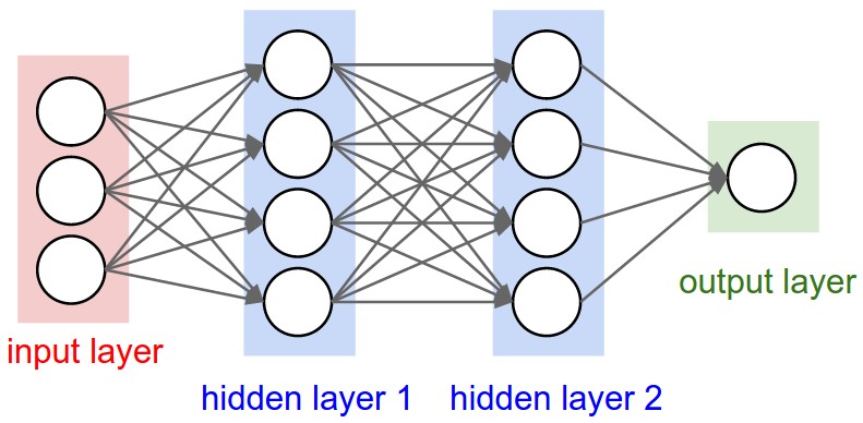
(Image Credit: Andrej Karpathy’s incredible notes for CS231N)

In the image above, we have an input with 3 dimensions. Lets call this $X$ . These three dimensions then go through a hidden layer, which performs the operation $W_1 X + b_1$ , where $W_1$ is a matrix of size 4x3 and $b_1$ is a vector of size 4 ( $W_1 X$ is a matrix multiplication). $W_1$ is also called a “weights matrix” as it effectively computes a bunch of weighted sums of elements in the vector. Recalling your matrix algebra, taking the product of a 4x3 matrix and a 3-dimensional vector yields a 4-dimensional vector. This output vector is, in theory, a new representation of the original input that presumably will help us with our task. For example, if we’re attempting the digit recognition task, the input could be the values of the pixels and the output of this hidden layer could be presence of certain curves or the angle of lines – “features” that help provide a higher-level understanding of the input data and the task. As the intuition goes, stacking these layers yields higher and higher feature representations. We then invoke some non-linear function on the result vector, say tanh. So the input to hidden layer 2 is just $tanh(W_1 X + b_1)$ . Each layer has its own matrix and vector pair, and we continue forwarding vectors through the neural net till we get the final output, which in our case is a single digit output. If we added signficantly more neurons to each layer (the circles in the diagram), we could use a similar architecture to train a task to recognize handwritten digits with the input being the values of the pixels on a grayscale and the output being the actual digit.

This is all great, but how do we get these magical weights in the first place? This is where the training process comes in. The approach is simple. First, we start with randomly initialized weights and forward a few examples through the net. Obviously, the results are not going to be good, but we can use the labels on the training data to get better. The idea is to have a “loss function” that gives us a sense of how far we are from the right answer. If the loss is high, our guess was way off, but if its low, our guess was pretty close to optimal. So we now have a way to grade our progress, but how do we learn from this? We can use good ol’ function optimization from calculus. If you recall from Math 51 or some other matrix calculus class, the gradient of a function is the direction of steepest ascent. So if you want to minimize an objective, like the loss function, we should go in the opposite direction of the gradient, or gradient descent. Hence, we to get our weights matrix, we can pass in an example, compute the loss, then compute the gradient of the loss with respect to the weights. This gives us a “step” in the right direction to a better set of weights, and we can update the weights accordingly. By doing this process repeatedly with different labeled examples, we can achieve highly optimized weights.

The process of computing this gradient can be quite laborious and error-prone by hand, but luckily many deep learning frameworks provide the ability to automatically compute gradients, and that’s exactly what this assignment focuses on.

Overview of DLang

Why DLang?

DLang exists to abstract away much of the details involved in implementing a deep learning model. As discussed above, deep learning often involves a variety of matrix operations, gradient calculations, and more. These can often be cumbersome to develop and implementations of these operations are often quite error-prone. The goal of DLang, like with many of the programming languages you have learned this quarter, is to abstract away the details involved in a nontrivial feature and make it almost impossible for an end user to make mistakes with regards to these features.

Specifically, the most salient features DLang provides are:

1) Easy and safe matrix and vector operations: In a typical imperative language, adding two vectors $A$ and $B$ would require you to loop over the elements in the vectors like so (in pseudocode):

A = [1, 2, 3, 4, 5]
B = [41, 40, 39, 38, 37]
if (A.length != B.length) raise Error
C = []
for (i = 0; i < A.length; i++) {
  C[i] = A[i] + B[i]
}

That’s a lot to write, and it’s quite easy to forget to check that the vectors are the same size before adding them. We’d much rather just write something like this:

A = [1, 2, 3, 4, 5]
B = [41, 40, 39, 38, 37]
C = A + B

2) Autodifferentiation for easy backpropagation: Deep learning models can involve arbitrarily complex loss functions with arbitrarily complicated gradients. It would be incredibly tiring to have to explicitly write a function for calculating the gradient of a long expression with respect to some target variable. Furthermore, if you’re like us and haven’t taken calculus since freshman year, you don’t want to be coding up gradients by hand – even for seasoned calculus aficionados, multi-variable gradient calculation is highly, highly error-prone. We’d rather have a simpler interface for calculating gradients that works on any arbitrary expression automatically, like so:

C = (A * B - 2) * 4
backwards(C, A)  // Gradient of C with respect to A; should be 4 * (A * B - 2) * B

Those of you familiar with Deep Learning will notice that the 1st feature is reminiscent of Numpy, a scientific computing library for Python with the ability to operate on n-dimensional arrays with ease, and that the 2nd feature is reminiscent of Pytorch, a deep learning framework for Python that (amongst other things) provides a vector-Jacobian product engine (read: calculates gradients without you having to think about it).

DLang Examples

Let’s go through a few quick example snippets to give you a general sense of how the language looks. We’ll do this in the style of learnxinyminutes.com (which, if you haven’t used it yet, is by far the quickest way to get to grips with a new language.)

(Note that this language does not actually feature an equality == operator; we only include this to show the results of operations.)

(* Defining Vectors, Matrices, and variables *)
(* Variable assignment is similar to python; no type or explicit declaration needed.
   Types are inferred via the typechecker. *)
X = Matrix[[10, 10, 10], [20, 20, 20], [30, 30, 30]];
Y = Vector[1, 2, 3];
A = 10;
B = -1;  (* Negative numbers are permitted. *)
C = 1.23;  (* Floats are permitted *)
D = 1.;  (* Number with a period is a float *)
W = Vector[1, 2.1, 3.12]; (* All numbers in a Vector/Matrix get coerced to float *)

(* Accessing Vectors and elements *)
X[1,1] == 20.;  (* Accessing a single element from a Matrix. Matrices and Vectors are 0-indexed. *)
X[1,] == Vector[20., 20., 20.];   (* Single index accessors on Matrices yield Vector slices *)
X[,1] == Vector[10., 20., 30.];
Y[,1] == 2.;  (* We can use either form of single index accessors on Vectors. *)
Y[1,] == 2.;

(* Performing element-wise binary operations *)
A + 5 == 15;
A + D == 11.;  (* Ints get coerced to float under a binop *)
Y * Vector[2, 2, 2] == Vector[2, 4, 6];  (* Binops executed element-wise *)
Z = Matrix[[1, 1, 1], [2, 2, 2], [3, 3, 3]];
X + Z == Matrix[[11, 11, 11], [22, 22, 22], [33, 33, 33]];  (* Binops executed element-wise *)

(* Performing matrix multiplications *)
ID = Matrix[[1, 0, 0], [0, 1, 0], [0, 0, 1]];
X @ ID == X;  (* Only defined on Matrices, cannot be applied on Vectors *)
X @ Matrix[[1, 1], [1, 1], [1, 1]] == Matrix[[30, 30], [60, 60], [90, 90]]

(* Function definition and application *)
(* Note that arguments must have types here. *)
def saxpy(a: num, X: Vector, Y: Vector) {
  a * X + Y;
}

saxpy(10, Vector[10, 10, 10], Vector[1, 2, 3]) == Vector[101, 102, 103];

(* Using built-in functions *)
numrows(X) == 3;  (* numrows and numcols return ints, not floats *)
numrows(Y) == 3;  (* numrows and numcols return the same value for Vectors *)
numcols(Y) == 3;
(* Second argument is the index to add the third argument at. *)
addrow(X, numrows(X), Vector[40, 40, 40]) == Matrix[[10, 10, 10], [20, 20, 20], [30, 30, 30], [40, 40, 40]];
addcol(Y, 1, 5) == Vector[1, 5, 2, 3];
sum(Vector[1, 2, 3]) == 6.;
sum(Matrix[[1, 2], [3, 4]]) == 10.;

(* A basic two layer NN computation *)
def two_layer_nn(X: Matrix, W1: Matrix, B1: Vector, W2: Matrix, B2: Vector) {
  H1 = W1 @ X + B1;
  return W2 @ tanh(H1) + B2;
}

At a high level:

DLang is a statement-based language, meaning a DLang program is a list of statements executed in order.
DLang only considers numbers, vectors, and matrices to be values.
DLang has two types of numbers: ints and floats.
- All numbers in Vectors and Matrices are coerced to floats.
- Any binary operation involving an int and a float involves a type coercion of the int to a float.
DLang provides a relatively minimal feature set: variables, top-level functions, and vector and matrix subscripting (i.e. accessing a subvector or element in a matrix or vector).
- Note that there are no strings, file I/O, loops, or even conditional statements. This is an extremely limited language designed to do exactly one thing and one thing only: do our matrix calculations and gradient computation.
DLang functions work more similarly to how they work in a traditional imperative language than what you’ve seen in functional languages in this class. That is:
- Functions are purely top-level constructs; they are not values and cannot be dynamically constructed, returned from functions, accepted as arguments to a function, or even be defined in another function.
- Functions effectively define lists of statements where the last statement in the list denotes the value “returned” from the function.
- There is no notion of void in this language, so all functions must return something.
- Just like in imperative languages, the arguments passed to a function are fully evaluated before they are injected into the function. That is, there is no lazy evaluation of arguments.
- Arguments are bound to the corresponding variables in the function signature. These variables are only in scope for the duration of the function. All variables are pass by copy.

Getting Started

From your CS 242 Git repo, run git pull and go to finals/dlang. If you have Python3.6+ and OCaml on your machine, you’re almost ready to go! If you’re on a Farmshare machine, use this Campuswire post to help you set up Python3.6+.

Run pip install -r requirements.txt to get our Python requirements, and type make in the project root directory to compile the OCaml code.

To ensure your starter code is valid, run cd tests && pytest -k DLangBase. This will run roughly 230 tests that cover the basic specification of the language – many of them are ones we used in the development of this project.

A Quick Tour of the Codebase

The codebase for this assigment is mostly in OCaml, and it’s actually quite reminiscent of the codebase you used in Assignment 4. The codebase defines the four components of an interpreter:

Lexer (lexer.mll): Defines a fancy regex that describes the valid tokens and symbols allowed in the language. This is the part that identifies errors like a stray parenthesis or an invalid variable name involving an emoji character.
Parser (grammar.mly): Defines a context-free grammar that describes what valid combinations of tokens are allowed in the language, and maps them to actual language constructs in an abstract syntax tree. This is the part that populated your Ast in assignment 4, and it helps us make sure that you use specific tokens only in ways that make sense. For example, in OCaml it doesn’t make sense to have an expression like f |10|, even though each token in this expression is a valid token used in OCaml (e.g. symbol, match pipe, and number).
Typechecker (typechecker.ml): You should be familiar with this one. The goal of the typechecker is to statically analyze the program and check for any violations of static semantic rules. For example, in OCaml, we shouldn’t allow "hello" / 5 even if it represents a valid formulation under the context-free grammar for OCaml. Ultimately, just because something is syntactically possible doesn’t mean it has any semantic meaning.
Interpreter (interpreter.ml): This actually executes the dynamic semantics of the language, and is responsible for “evaluating” a program. You should be familiar with this stage too.

If you would like some more background on these four components, check out this short slide deck from CS 143 (which is a fantastic class to follow up CS 242 with!)

In this project, you’ll get the chance to engage with all four stages of the interpretation process, with most of the emphasis on the interpreter and typechecker.

Using the interpreter and test suite.

You can interpret any arbitrary DLang program by doing ./main.native test.dl (where test.dl is your program). You can also do ./main.native -lp ... to run just the lexer and parser, and ./main.native -t ... to run only up to the typechecker.

We use the pytest testing framework for this project. Check out their docs if you need help installing, running tests, or adding your own tests. It may help to read about pytest fixtures if you intend on reading through the suite or adding tests.

Task 1: Introduce Matrices to DLang (25%)

This first task is designed to help you get your bearings in our codebase. While we have shown you examples of DLang programs involving Matrices, they actually aren’t a supported feature in the version of DLang provided in your starter code. For this first task, you’ll need to implement 4 main features:

Defining Matrices
Accessing specific elements in a Matrix given a row and column coordinate.
Performing Matrix Multiplications (If you need a refresher on this operation, check here.)
Extending element-wise binary operations and builtins to work on Matrices.

As you’ll notice, Matrices appear nowhere in the codebase. This means you’ll need to implement them from scratch and add support for them over all four components of the interpreter. Specifically, you’ll need to make sure a program like the following works with the prescribed syntax:

def f(x: Matrix, y: Vector) {
  x[1,] + y;
}

m = Matrix[[1]];
m = addcol(m, 1, Vector[1]);
m = addrow(m, 1, Vector[1, 1]);
v = Vector[42, 42];
f(m @ m + m, v)[0,] + m[numrows(m) - 1, numcols(m) - 1] + sum(m);

(If you’re curious, this should output 50.)

While you have experience with OCaml typecheckers and interpreters from Assignment 4, the lexer and parser may be new to you. OCaml actually has first-class support for OCamllex and Menhir, which provide easy lexing and parsing utilities. You can read more about their usage here:

A few tips and notes:

You are free to implement Matrices however you want, so long as you obey the syntax and semantics defined above.
Matrix[[]] is considered to be an empty matrix with dimensions 0x0.
We’ve generously left the full implementation of Vectors in the starter code, so you can also use this to help implement Matrices.
We suggest you use OCaml Array to implement your Matrix instead of List as Arrays provide O(1) random access to elements. Also, elements can be updated in place. This means it may make sense to occasionally use more imperative code instead of using functions that involve duplicating the full array.
The tests for the components are under the test suite classes prefixed with TestMatrix..., located in tests/test_lexer_parser.py, tests/test_typechecker.py, and tests/test_interpreter.py.

Testing

To test your implementation of Matrix and the associated operations, you can run cd tests && pytest -k "Matrix" from the project root directory. If all tests pass, you are guaranteed full marks for this part of the assignment. There are no hidden tests for this task.

Task 2: Write a built-in convenience function to generate matrices (5%)

DLang includes a special set of privileged functions that are built in to the language’s core. These functions have interfaces in DLang, but are actually executed in OCaml. The rationale here is that there are some functions that a) can’t be written without having access to the underlying implementation of the language, and/or b) way too computational expensive to implement in the actual language. This is a relatively common concept, with languages like Python implementing a set of core built-ins in some lower level language (e.g. C, Java), and then implementing the rest of the language using those built-ins.

For DLang, we provide built-ins like numcols and numrows, which can be used to get the shape of a tensor, and addrow and addcol, which can be used to dynamically change the shape of a tensor.

During training for a deep learning model, we often need to start off by randomly initializing a matrix of weights for each layer of the neural net. While addrow and addcol do give us the ability to dynamically add rows and columns to a tensor in DLang, it can be cumbersome to generate, say, a $768 \times 256$ matrix, especially given that we have no loop constructs in DLang. Hence, you’re tasked with making two tensor creation built-ins to provide some more convenience to DLang.

Namely, we’d like you to build:

rand(r, c), which generates an $r \times c$ Matrix with random values between 0 and 1.
fill(r, c, val), which generates an $r \times c$ Matrix with all elements set to val.

Testing

Run cd tests && pytest -k "BuiltinsCreation" and cd tests && pytest -k "MatmulTiming" from the project root directory.

If all tests pass, you are guaranteed full marks for this part of the assignment. There are no hidden tests for this task. That being said, the tests are not exhaustive, and we highly suggest you write additional tests.

If tests in the MatmulTiming suite fail, this means your rand or matmul implementation is too slow. If you’re running into issues here, make sure you’re exploiting the fact that Arrays let you update elements in-place.

Task 3: Implement autodifferentiation for scalars (35%)

Now it’s time for the big leagues! We’re going to implement the jewel in the crown for DLang: autodifferentiation. As mentioned above, autodiff allows us to programatically compute the gradient of a given expression with regard to some variable.

Chain Rule Review

(If you’re familiar with chain rule and backpropagation, you can feel free to skip this).

It’s worth considering why this is possible in the first place. Recall the chain rule that forms the backbone of backpropagation. The chain rule is quite powerful, since it effectively gives us a way to decompose any arbitrarily complex gradient into a couple of simple, easily programmable building blocks, and tells us to how combine those building blocks. For example, $c = 3 * a + 15$ can be decomposed as such:

$\begin{align*} b &= 3 * a \\ c &= b + 15 \end{align*}$

In order to compute $\frac{\partial c}{\partial a}$ , we can compute $\frac{\partial c}{\partial b} \times \frac{\partial b}{\partial a}$ . And fortunately, we have well-defined rules for calculating these subexpressions. Going back to Calculus I, we can invoke the sum and product rules, which state that:

$\frac{\partial}{\partial x}(y + z) = \frac{\partial y}{\partial x} + \frac{\partial z}{\partial x} \\ \frac{\partial}{\partial x}(y \times z) = \frac{\partial y}{\partial x} z + y \frac{\partial z}{\partial x}$

Hence, in the example above, we have that:

$\begin{align*} \frac{\partial c}{\partial b} &= \frac{\partial}{\partial b} (b) + \frac{\partial}{\partial b} (15) = 1 + 0 = 1 \\ \frac{\partial b}{\partial a} &= \frac{\partial}{\partial a} (3) \times a + 3 \times \frac{\partial}{\partial a} (a) = 0 + 3 = 3 \\ \frac{\partial c}{\partial a} &= \frac{\partial c}{\partial b} \times \frac{\partial b}{\partial a} = 3 \end{align*}$

This is remarkable: we have the ability to compute virtually any gradient by just computing gradients over a single operation and combining them via multiplication. This means that if we have a way of capturing the graph of computation for a given expression, we can easily compute the gradient with respect to some variable just by walking the graph!

Forward- vs Reverse-Mode Autodifferentiation

Now that we’ve established that chain rule allows us to use the computation graph for an expression to compute its gradient, we now have two options:

Compute the gradient as we compute the “forward pass” of the expression. This is called “forward-mode autodiff.”
Compute the gradient after we have computed the “forward pass” by walking backward through the computation graph. This is called “reverse-mode autodiff.”

Another way of thinking about this is that chain rule specifies a gradient to be the product of other gradients. We can either compute these gradients in forward order, i.e.: $\frac{\partial z}{\partial x} = \frac{\partial y}{\partial x} \times \frac{\partial z}{\partial y}$ , or in reverse order (which may be the more familiar formulation from your intro calculus classes), i.e. $\frac{\partial z}{\partial x} = \frac{\partial z}{\partial y} \times \frac{\partial y}{\partial x}$ . Both approaches are mathematically equivalent due to commutativity of multiplication, but computationally they involve different strategies for implementation.

For forward-mode, we can imagine replacing each variable of interest $x$ in the computation graph with a “dual number” $\langle x, x' \rangle$ , where we keep track of the forward pass arithmetic on the left and the gradient arithmetic on the right. Hence, when computing the value of $c$ (forward pass) in the following example:

$\begin{align*} b &= 3 \times a \\ c &= b * b \\ d &= c + 15 \end{align*}$

we could keep track of the accumulated gradient with respect to $a$ in the right of each dual while calculating the forward pass in the left as so:

$\begin{align*} b &= \langle 3, 0 \rangle \times \langle a, 1 \rangle \\ c &= \langle 3 \times a, 3 \rangle \times \langle 3 \times a, 3 \rangle \\ d &= \langle 9 \times a^2, 18 \times a \rangle + \langle 15, 0 \rangle \\ &= \langle 9 \times a^2 + 15, 18 \times a \rangle \end{align*}$

The key idea is that while we evaluate the expressions, we can also compute their gradients with respect to variables of interest simultaneously by using basic building block rules (e.g. sum rule and product rule).

The above is a quick example. For the rules involved in adding dual numbers, check page 7 of this paper. You’ll also need to consider some other complexities: for example, how would you generalize the notion of duals to handle the case where multiple variables need to be gradient-tracked? There’s a variety of legitimate ways to do this, and figuring out a viable technique will be part of your challenge.

For reserve-mode, we compute the forward pass and cache the values of each intermediate node in the computation. From there, we can calculate the gradient using the cached values. For instance, in the same example as above, we might compute the values of $b$ , $c$ , and $d$ and cache them. Then we can compute the gradient as follows:

$\begin{align*} \frac{\partial d}{\partial c} = 1 && \frac{\partial c}{\partial b} &= 2b = 6a && \frac{\partial b}{\partial a} = 3 \\ \frac{\partial d}{\partial a} &= \frac{\partial d}{\partial c} \times \frac{\partial c}{\partial b} \times \frac{\partial b}{\partial a} = 18a \end{align*}$

For the rules involved in computing the partial gradients above, check page 4 of this paper.

We encourage you to go through the following resources to start gaining an intuitive understanding:

The Wikipedia article on Autodiff
This paper by Wang et al. that takes a PL-theoretic view of autodiff and includes some great dynamic semantic rules
This slide deck from CS231N on backpropagation (check out slides 36 to 94 for some fully worked examples!)

Your task

While both forward-mode and reverse-mode autodiff yield the same result, they each have their own complexities and tradeoffs when implemented in a concrete computational system. It is up to you to determine how you want to design and develop your autodiff feature. Our only requirement is that it works with the following syntax:

x: track_grad = 1;
y = x * 3;
z = y * y + y;
backward(z);
grad(x);  (* returns 21.0 *)

where:

track_grad is a tag on a variable indicating DLang should keep track of the gradient with respect to the variable. We’ll refer to gradient-tracked variables as “dvars” for simplicity. If we say “gradient for a dvar x”, we mean “gradient with respect to x”.
backward(expr) is a built-in function that tells DLang to compute the gradient of expr for all dvars that are part of the computation graph for expr. If backward is called multiple times, sum the gradients on all dvars involved in the expression. backward itself has no meaningful return value; it is simply used for its side-effects. While the exact contents of backward depend on the mode of autodiff you choose, you should maintain this invariant: Calling grad on a dvar yields the sum of the gradients for the dvar computed on each expression passed to backward. More on this below.
grad(var) is a built-in function that returns the accumulated gradient of some dvar var as a float.

Specifically, you’ll need to support autodiff on programs involving: ints, floats, scalar binary operations, variable assignments, and functions that accept and return scalars.

Ultimately, this task is quite open-ended and you’re free to pursue any implementation that allows you to pass the tests. However, to provide a little more guidance, we suggest a general approach like the following to get started.

Add support for the track_grad symbol at the lexer and parser level.
Add some way of distinguishing between dvars and regular variables. There’s a couple ways to do this, like adding more fields to relevant Ast records or adding some kind of map from variable name to a bool.
Implement a barebones version of autodiff: while we eventually expect you to have autodiff on a whole variety of expressions, it may be easier to first implement autodiff for some barebones subset of expressions, like ints, floats, and additions.
- For forward-mode: add some kind of Dual type to the Ast and then edit your eval_expr and eval_stmt functions to do gradient calculations along with the expression evaluation.
- For reverse-mode: add some new function that recursively computes gradients by walking through an Ast. Since eval_expr and expr_stmt eargly evaluate expressions, you may lose some crucial info (e.g. the expression a variable was initially bound to). You’ll need to find some way to track that info so you can use it in your new gradient function.
Add support for backward as a builtin at the lexer, parser, and typechecker level.
Add interpreter support for the backward builtin. For forward-mode, backward will likely do minimal work since you eagerly compute gradients during expression evaluation. For reverse-mode, backward will likely invoke your new gradient function. In both cases, you’ll need to figure out some way to identify all the dvars in the expression and store the gradients for these dvars in some place you can retrieve from later.
Lexer, parser, typechecker, and interpreter support for grad. grad will likely do very little, as it mainly just needs to look up the gradient for a dvar. The main development work involved here is ensuring you have some way of storing and accessing gradients after they’re computed.

Once you’ve built up this infrastructure, you should now have all the major pieces in place for implementing the rest of autodiff. At this point, you can adopt an iterative approach to development by gradually adding in support for other types of expressions. We STRONGLY SUGGEST developing in this iterative fashion – autodiff is a non-trivial feature to implement and implementing it all at once is unlikely to be a winning strategy.

Examples and Rules

Since the behavior of autodiff can be complex, here’s a few concrete rules and example programs to help guide you. You’re also welcome to look through the test suite, which features examples with nuanced behavior also.

First off, some rules you may remember from intro calculus. To keep things simple, we use $\frac{d}{dx} e$ to represent a gradient of expression $e$ with respect to dvar $x$ . When you implement your autodiff, you’ll need to handle cases where there’s multiple dvars (more on this below).

$\begin{align*} \ir{D-Sum-Rule} {} {\steps{\frac{d}{dx}(e_1 + e_2)}{\frac{d}{dx} e_1 + \frac{d}{dx} e_2}} \s \\ \ir{D-Difference-Rule} {} {\steps{\frac{d}{dx}(e_1 - e_2)}{\frac{d}{dx} e_1 - \frac{d}{dx} e_2}} \s \\ \ir{D-Product-Rule} {} {\steps{\frac{d}{dx}(e_1 * e_2)}{\frac{d}{dx} e_1 \times e_2 + e_1 \times \frac{d}{dx} e_2}} \s \\ \ir{D-Quotient-Rule} {} {\steps{\frac{d}{dx}(e_1 / e_2)}{\frac{\frac{d}{dx} e_1 \times e_2 - e_1 \times \frac{d}{dx} e_2}{e_2 * e_2}}} \s \end{align*}$

And some more specific rules for DLang: $\begin{align*} \ir{D-Var} {y = e;} {\steps{\frac{d}{dx}(y)}{\frac{d}{dx}(e)}} \s \ir{D-Func} {def f(x, ...) {...; e;} } {\steps{\frac{d}{dx}(f(x, ...))}{\frac{d}{dx}(e)}} \s \end{align*}$

(An english translation of the D-Func rule is that the gradient of a function application for some dvar is the same as the gradient of the last statement – the ‘return’ statement – of the function for that dvar.)

Now for some examples. Here’s a simple case with binary operations:

x: track_grad = 10;
backward(x * 2 + 5); (* Gradient for x is 2. based on sum and product rules *)
grad(x);  (* returns 2. This value is presumably stored somewhere easily accessible
             after the call to backward. *)

Dvars can be invoked multiple times:

x: track_grad = 10;
y = x + 5;  (* Gradient for x is 1. *)
z = x * 2;  (* Gradient for x is 2. *)
backward(y + z); (* When backpropagating through y + z, we encounter two references to x.
                    We should compute dy/dx and dz/dx separately, then combine them with
                    the sum rule. *)
grad(x);  (* returns 3. *)

Variable assignments should allow gradients to flow through their bound expression, even if the variable itself is not gradient-tracked.

x: track_grad = 10;
y = x * 2;  (* Even though y is not a dvar, x is, and we should backpropagate through the expression x * 2. *)
            (* Gradient of y with respect to x is 2. *)
z = y * 5;  (* Similarly, gradient should flow through this assignment too. *)
            (* Gradient of z with respect to y is 5. *)
backward(z); (* equivalent to backward(x * 2 * 5) *)
            (* Gradient of z with respect to z is 1. *)
grad(x);  (* returns 10., by chain rule: dz/dx = dz/dy * dy/dx *)

However, if a variable is rebound, you only need to backpropagate to the last rebinding.

x: track_grad = 10;
x: track_grad = x * 2;  (* Since we rebound `x`, calls to `backward` will only
                         backpropagate to this point when computing the gradient for x. *)
backward(x * 5);
grad(x);  (* returns 5. *)

For function calls involving dvars in the argument expressions, compute the gradient through the function statements.

def f(x: float) {
  y = x * 2;
  y + 5;  (* We should backpropagate through statements in reverse order, so we start here. *)
}

x: track_grad = 10;
backward(f(x));  (* equivalent to backward(x * 2 + 5) *)
grad(x);  (* returns 2. *)

If backward is called on an expression involving multiple dvars, compute gradients for each one. This may require you to use the evaluated value of the dvars (here we need to use the fact that y = 5 and x = 10).

x: track_grad = 10;
y: track_grad = 5;
z = x * y + 2;
backward(z);  (* expression involves 2 gradient-tracked variables *)
grad(x);  (* returns 5., the gradient of xy + 2 for x given y = 5. *)
grad(y);  (* returns 10., the gradient of xy + 2 for y given x = 10. *)

If some dvar is involved in the expression for multiple calls to backward, sum the gradients calculated.

x: track_grad = 10;
backward(x * 5);  (* gradient for x is 5 for this expression. *)
backward(x * 10);  (* gradient for x is 10 for this expression. *)
grad(x);  (* returns 15.0, the sum of 5. and 10. *)

Whew! Before you go off to the races, here’s a few tips:

If you intend on using the Ast to store some extra info, it may help to look into refs and mutable fields in OCaml.
You are free to change virtually any part of the DLang implementation to make your implementation easier. It’s an open ended problem and you can use whatever means necessary to achieve your goal here, as long as the tests pass and you don’t break other functionality.
Just in case we didn’t say it enough: design, develop, and test ITERATIVELY. Try one thing at a time, see what works and doesn’t work, and keep iterating till you having working functionality. While it’s valuable to think over this a bit, focus on getting some code out; do not try to come up with the full design on paper in one go.
If you’re confused about the behavior for autodiff, or you just want a sandbox to play in, consider loading up Pytorch in the Python interpreter. (The latest version of requirements.txt includes a pytorch installation. Relevant Pytorch docs available here.) Here’s a sample program you could use to explore some autodiff behavior:
```
  import torch
  x = torch.tensor(5., requires_grad=True)
  (x * 2).backward()
  x.grad
```
You’ll notice there’s significant similarities between DLang’s and Pytorch’s autodiff-related operations. This is not merely coincidence, and in most cases, the behavior across the two should be similar. Notable exceptions are in the FAQ below.

FAQ

What if a program calls grad on some variable not tagged with track_grad?
- You should throw an error in the typechecker.
What if a program calls grad on some variable that has yet to accumulate a gradient (i.e. no call to backward has involved the variable in question)?
- Technically, we’d want to return no value, but since our language has no notion of void, we’ll permit any behavior that results in a float value being returned. For example, a reasonable thing to do would be to return 0.0.
- Our language has no notion of void since this makes the implementation a bit cleaner for you. If we were actually releasing DLang to the world, it would be useful to include a void type, but since this is just a pedagogical tool, it’s not very enlightening to add void to the language.
What does backward return?
- backward is only used for its side-effects, but since our language lacks a void type, you’re allowed to return any value you like. We will never use the return value of backward in an expression.
- You are also permitted to add a void type if you really, really want to. Just make sure you still pass the tests.
How do you compute the gradients through builtin functions?
- You don’t have to. backward should refuse to compute the gradient of an expression containing a builtin. In fact, such a program should not even typecheck. To be clear, the following program should not pass the typechecker:
```
  x = Vector[1, 2];
  backward(numcols(x));
  grad(x);
```
  That being said, if a builtin isn’t involved in the expression you wish to compute gradients on, it’s allowed. For example,
```
  x:track_grad = sum(Vector[1.]);
  backward(x * 2);
  grad(x);
```
  is still perfectly valid since we only need to compute gradients with respect to x; we never need to backpropagate through the rand builtin and actually stop right before then.
Does track_grad persist across variable rebindings?
- No. That is, for a program like the following:
```
   x:track_grad = 5;
   a = x;
```
  a is not a gradient-tracked variable, and calls to backward should not compute gradients with respect to a (although they should compute gradients with respect to x.)
Can function signatures include track_grad?
- No. Programs like this are disallowed at the parser level:
```
   def f(a: track_grad : int) {
      a + 5;
   }
   x = 5;
   f(x);
```
  If you want to track the gradient through f, tag the input argument with track_grad (x in this case). (Note that track_grad is still perfectly valid in a function body.)

Testing

To test your implementation autodifferentiation for scalars, you can run cd tests && pytest -k "AutodiffScalar" from the project root directory.

All tests are provided and there are no hidden tests.

Task 4: Implement autodifferentiation for Vectors and Matrices (25%)

Now that you’ve put in all the elbow grease getting the infrastructure for autodiff in Task 3, all you need to do is generalize some of the logic to work for Vectors and Matrices and support a few other features. Specifically this entails three subtasks:

1) Supporting autodiff on element-wise binary operations for Vectors and Matrices. 2) Supporting autodiff on row, column, and element accessors on Vectors and Matrices. 3) Supporting autodiff on matrix multiplication.

(Other features, like autodiff on functions, should work with Matrices/Vectors in the function args and body with little extra effort if your implementation is correct.)

Let’s go through some examples of the expected behavior of these three features, followed by some concrete rules.

Element-wise Binary Operations

First, let’s look at element-wise binary operations:

x:track_grad = Vector[1, 1, 1];
backward(x * Vector[2, 4, 6]);
grad(x);  (* returns Vector[2., 4., 6.] *)

As shown above, we take a vector x and multiply it element-wise with another vector. Since each element in the original vector x is being multiplied by different numbers in line 2, they each have different rates of change from a mathematical perspective, and hence different gradients. This implies that each element in the original vector should have its own gradient, and that’s exactly what happens above. Specially, since the element with index 0 in x gets multiplied by 2, the gradient with respect to that element is just 2. Similarly, since the element with index 1 in x gets multiplied by 4, the gradient with respect to that element is 4. This underlies a key intuition for this assignment: the gradient of some expression with respect to some vector/matrix x has the same shape (i.e. same dimensions) as x itself (note that this is not true with all matrix calculus in general; it’s only under the conditions guaranteed by the assignment. An explanation is provided below if you’d like to learn more, but it’s not necessary for this assignment.) This logic can also be very intuitively translated to Matrices.

If the above is a bit confusing still, consider the following program, which is identical in output to the program above.

x0:track_grad = 1;
x1:track_grad = 1;
x2:track_grad = 1;
backward(2 * x0);
backward(4 * x1);
backward(6 * x2);
Vector[grad(x0), grad(x1), grad(x2)]; (* returns Vector[2., 4., 6.] *)

More formally, we have the following rules governing element-wise binary operation autodiff. $\oplus$ represents the four element-wise binary operations.

$\begin{align*} \ir{D-Vector-Binop} {v = Vector[v_0, v_1, ..., v_n]; u = Vector[u_0, u_1, ..., u_n];} {\steps{\frac{d}{dv}(v \oplus u)}{Vector[\frac{d}{dv_0} v_0 \oplus u_0, \frac{d}{dv_1} v_1 \oplus u_1, ..., \frac{d}{dv_n} v_n \oplus u_n]}} \s \\ \ir{D-Matrix-Binop} {s = Matrix[[s_{00}, ..., s_{0n}], ..., [s_{m0}, ..., s_{mn}]]; t = Matrix[[t_{00}, ..., t_{0n}], ..., [t_{m0}, ..., t_{mn}]];} {\steps{\frac{d}{ds}(s \oplus t)}{Matrix[[\frac{d}{ds_{00}} s_{00} \oplus t_{00}, \frac{d}{ds_{0n}} s_{0n} \oplus t_{0n}], ... [\frac{d}{ds_{m0}} s_{m0} \oplus t_{m0}, ..., \frac{d}{ds_{mn}} s_{mn} \oplus t_{mn}]]}} \s \end{align*}$

Accessors

Now let’s consider accessors under autodiff:

x:track_grad = Vector[1, 1, 1];
y = x[1,] * 4;
backward(y);
grad(x);  (* returns Vector[0., 4., 0.] *)

In the example above, the only part of the Vector x that actually contributes to the expression we call backward on is the element with index 1. Hence, by the definition of a gradient, the rate of change of the y given a change in the 0th or 2nd elements is 0, since they don’t even factor into the calculation. Accessors are gradient-blockers: they restrict the flow of gradient to just the selected elements.

Since there’s multiple types of accessors available for matrices, the behavior can be a bit more nuanced:

m:track_grad = Matrix[[1, 1], [1, 1]];
backward(m[0,] * 2);
backward(m[,0] * 2);
backward(m[0,0] * 4);
grad(m);  (* returns Matrix[[8., 2.], [2., 0.]] *)

In this case, the element at index 0, 0 is involved in three of the expressions we call backward on, and hence it accumulates a gradient of 8. Meanwhile the elements at 0, 1 and 1, 0 accumulate gradients through only one of the expression. Finally, the element at 1, 1 is not involved in any of the expressions, so it gets 0 accumulated gradient.

More formally:

$\begin{align*} \ir{D-Vector-Row-Accessor} {v = Vector[v_0, v_1, ..., v_n];} {\steps{\frac{d}{dv}(v[i,])}{Vector[0.0, ..., 1.0 \text{(at the } i \text{th index)}, ..., 0.0]}} \s \\ \ir{D-Vector-Col-Accessor} {v = Vector[v_0, v_1, ..., v_n];} {\steps{\frac{d}{dv}(v[,i])}{\frac{d}{dv}(v[i,])}} \s \\ \ir{D-Matrix-Row-Accessor} {s = Matrix[[s_{00}, ..., s_{0n}], ..., [s_{m0}, ..., s_{mn}]];} {\steps{\frac{d}{ds}(s[i,])}{Matrix[[0., ..., 0.], ..., [1., ..., 1.] , ..., [0., ..., 0.]];}} \s \\ \ir{D-Matrix-Col-Accessor} {s = Matrix[[s_{00}, ..., s_{0n}], ..., [s_{m0}, ..., s_{mn}]];} {\steps{\frac{d}{ds}(s[,j])}{Matrix[[0., ..., 1., ... 0.], ..., [0., ..., 1., ... 0.]];}} \s \\ \ir{D-Matrix-Elem-Accessor} {s = Matrix[[s_{00}, ..., s_{0n}], ..., [s_{m0}, ..., s_{mn}]];} {\steps{\frac{d}{ds}(s[i,j])}{Matrix[[0., ..., 0.], ..., [0., ..., 1., ... 0.], ... [0., ..., 0.]];}} \s \\ \end{align*}$

Matrix Multiplication

Finally, let’s consider matrix multiplication. While this may seem like the hardest, thanks to some linear algebra magic, it may actually be the easiest. It turns out that under certain conditions (once again feel free to read the Appendix below if curious), the following statements hold. Assume $A$ is a matrix of dimensions $m \times n$ and $B$ is a matrix of dimensions $n \times p$ .

$\begin{align*} \frac{d}{dA} A @ B &= \mathbf{1} @ B^T \\ \frac{d}{dB} A @ B &= A^T @ \mathbf{1} \end{align*}$

where $\mathbf{1}$ is a matrix of all ones with dimensions $m \times p$ and $A^T$ denotes the matrix transpose of $A$ . One potentially useful rule to know about transposes: for some matrix multiplication $A @ B$ , $(A @ B)^T = B^T @ A^T$ .

That’s right! That’s all there is to it. Let’s see some concrete examples:

x: track_grad = Matrix[[1., 2.], [3., 4.]];
y: track_grad = Matrix[[1., 0.], [0., 1.]];
backward(x @ y);
grad(x);  (* returns Matrix[[1., 1.], [1., 1.]] *)
grad(y);  (* returns Matrix[[4., 4.], [6., 6.]] *)

Finally, let’s see one example with a chained matrix multiplication involving matrices of varying dimensions:

x: track_grad = Matrix[[1., 1.], [1., 1.], [1., 1.]];  (* 3x2 matrix *)
y: track_grad = Matrix[[1., 0.], [0., 1.]];  (* 2x2 matrix *)
z: track_grad = Matrix[[1., 2., 3., 4.], [5., 6., 7., 8.]];  (* 2x4 matrix *)
backward((x @ y) @ z);
grad(x);  (* returns Matrix[[10., 26.], [10., 26.], [10., 26.]] = 1 @ (y @ z)^T = 1 @ z^T @ y^T *)
grad(y);  (* returns Matrix[[6., 14.], [6., 14.]] = x^T @ 1 @ z^T *)
grad(z);  (* returns Matrix[[2., 2.], [2., 2.]] = (x @ y)^T @ 1 = y^T @ x^T @ 1 *)

Note that in each case, the matrix dimensions work out for computing the gradient. That is:

For grad(x), we have $\mathbf{1} @ z^T @ y^T$ , where $\mathbf{1}$ is 3x4, $z^T$ is 4x2, and $y^T$ is 2x2. Hence, looking at the dimensions, we have (3x4) @ (4x2) @ (2x2), yielding 3x2 like expected.
For grad(y), we have $x^T @ \mathbf{1} @ z^T$ , where $x^T$ is 2x3, $\mathbf{1}$ is 3x4, and $z^T$ is 4x2. Hence, looking at the dimensions, we have (2x3) @ (3x4) @ (4x2), yielding 2x2 like expected.
For grad(z), we have $y^T @ x^T @ \mathbf{1}$ , where $y^T$ is 2x2, $x^T$ is 2x3, and $\mathbf{1}$ is 3x4. Hence, looking at the dimensions, we have (2x2) @ (2x3) @ (3x4), yielding 2x4 like expected.

Your task + tips

In a nutshell, your task is to implement the above three features in your autodiff implementation. While the exact technique for implementation depends on how you chose to implement autodiff, we suggest breaking down the task either by type or by feature. That is:

By type: Implement vector binary operations, then row/col accessors for vectors, then matrix binary operations, then row/col/elem accessors for matrices, etc.
By feature: Implement vector binary operations, then matrix binary operations, then row/col accessors for vectors, then row/col/elem accessors for matrices, etc.

Here’s some tips:

If you’re using Pytorch as a sandbox for exploring autodiff behavior, you’ll need to write your code slightly differently for getting gradients on vector- or matrix-valued expressions:

For vector-valued expressions passed to backward:
```
  x = torch.tensor([1., 2., 3.], requires_grad=True)
  y = x * 2
  y.backward(torch.ones(y.shape[1]))
  x.grad
```
For matrix-valued expressions passed to backward:
```
  x = torch.tensor(([1., 2.], [3., 4.]), requires_grad=True)
  y = x.matmul(torch.tensor([[1., 0.], [0., 1.]]))
  y.backward(torch.ones(x.shape[0], y.shape[1]))
  x.grad
```
This is because you need to supply the gradient “seeds” to Pytorch so it knows what gradients to backpropagate. Read more in the Appendix if you’re curious why this is needed.

Testing

To test your implementation autodifferentiation for tensors, you can run cd tests && pytest -k "AutodiffTensor" from the project root directory.

The command above will run all the tests for autodiff on matrices and vectors, and is useful when you are done with the task. However, in order to support type-major or feature-major approaches to developing this task, we’ve split this test suite into 6 smaller suites:

TestAutodiffTensorElemwiseVectors
TestAutodiffTensorElemwiseMatrices
TestAutodiffTensorAccessorsVectors
TestAutodiffTensorAccessorsMatrices
TestAutodiffTensorMatrixMultiply
TestAutodiffTensorComposite: tests that consider interaction of matrices, vectors, scalars, and functions. The ultimate test of your implementation.

To run any of the above suites, just run pytest -k "<TEST SUITE HERE>".

Like above, all tests have been provided and there are no hidden tests.

Extension Tasks

Once you’ve completed your base assignment, you can have the option of completing some extra extensions to make DLang more awesome and usable. Completing an extension can grant you extra credit on the assignment depending on your correctness and progress. The maximum extra credit is listed next to the extension name. If you attempt both, your extra credit is capped at 15%. It is possible to get partial credit on extensions.

If you choose to do extra credit, please create a separate copy of your working DLang src directory called broadcast-src or inference-src and make your changes there. This will ensure that if you introduce regressions on other features while implementing your extensions, it will not harm your grade. Should you intend on doing both extensions, please make separate implementations for them – combining these two features is highly non-trivial.

Finally, if you intend on attempting these extensions, please DM either Sicheng or Shrey on Campuswire so we can get a sense of who’s doing which extensions.

Broadcasting (max 15% extra)

You may have noticed it’s a bit annoying to do some seemingly basic tasks in DLang, like adding a scalar to a Matrix. To do this, you’d actually have to generate a whole Matrix filled with the scalar value, like this:

def add_scalar(a: Matrix, b: int) {
  m = fill(numrows(a), numcols(a), b);
  a + m;
}

However, it would be much nicer if we could just do:

def add_scalar(a: Matrix, b: int) {
  a + b;
}

and have the scalar b added to each element of a.

This is called broadcasting, and is implemented by virtually all the major matrix-processing libraries, including Numpy and Pytorch. First, we suggest reading this short article on broadcasting in Numpy.

For this extension, we would like you to specifically implement broadcasting for three specific situations:

Scalar and Vector under a binary operation, e.g. 2 + Vector[10, 10] => Vector[12, 12]
Scalar and Matrix under a binary operation, e.g. 2 * Matrix[[10, 10], [10, 10]] => Matrix[[20, 20], [20, 20]]
Matrix and Vector under a binary operation, e.g. Matrix[[10, 10], [5, 5]] / Vector[5, 5] => Matrix[[2, 2], [1, 1]].

While the first two are fairly straightforward, the last one merits some more consideration. Let’s say we have:

Matrix[[10, 10], [5, 5], [0, 0]] / Vector[5, 5, 5, 5];

This would be an invalid broadcast, since there’s no logical way to divide a 4-dimensional vector from a 3x2 vector.

On the other hand, in a case like this, we’ve got some ambiguity:

Matrix[[10, 10], [5, 5]] / Vector[5, 1];

Do we do an element-wise division on a row-by-row basis (e.g. [10, 10] / [5, 1]) or column-by-column basis (e.g. [10, 5] / [5, 1]). Both yield different results. Most matrix libraries resolve this by arbitrarily dividing along the last dimension, which in our case is along the row. Hence, we should output Matrix[[2, 10], [1, 5]] in the example above.

Finally, there’s cases where only one dimension makes sense for broadcasting:

Matrix[[10, 10, 10], [5, 5, 5]] / Vector[10, 5]

In this case, we can only divide column-by-column since we we can’t divide a 3-dimensional row from the vector by the 2-dimensional vector provided. Hence we should get Matrix[[1, 1, 1], [1, 1, 1]] from the above.

Note that to get full credit here, you’ll need to also ensure your approach works on autodiff too, i.e. doing:

x:track_grad = Vector[1, 2, 3];
backward(x + 2);
grad(x);

is equivalent to:

x:track_grad = Vector[1, 2, 3];
backward(x + Vector[2, 2, 2]);
grad(x);

To test your implementation, run pytest -k Broadcasting for some basic tests. Hidden tests will be run after the assignment deadline is passed.

Type Inference (max 10% extra)

Currently, DLang relies on static type tags in function signatures like this:

def f(a: int, b: float, c: Vector) {
  a + b * c[0,];
}
f(10, 5.0, Vector[1, 2, 3]);

However, during the typechecking phase, you can actually infer the types of the function based on the arguments passed to the function. For example, in the case above, we can infer that the types are int, float, and Vector just by observing what’s passed to function f.

In this extension, you’ll aim to make DLang type safe while making it so programmers don’t need to explicitly provide types to DLang. That is, you’ll aim to allow programmers to write a program in DLang like this (look ma, no types!):

def f(a, b, c) {
  a + b * c[0,];
}
f(10, 5.0, Vector[1, 2, 3]);

Of course, type inference doesn’t give you a free pass on type safety. Here’s some examples of bad programs you’d have to suss out.

Below, we see two invocations of f. The first one uses valid operations and should cause the typechecker to set f to have a signature of (a: int, b: float, c: Vector). The second invocation supplies the wrong args given this implied type.

def f(a, b, c) {
  a + b * c[0,];
}
f(10, 5.0, Vector[1, 2, 3]);  (* f signature is now (int, float, Vector) *)
f(10, Vector[2, 3], Vector[1, 2, 3]);  (* `b` must be a float *)

Here we see a case where we end up performing an invalid operation in the function body given the argument types.

def f(a, b, c) {
  a + b * c[0,];
}
f(10, 5.0, Matrix[1, 2, 3]); (* Even though `c` still has a row accessor, it
                                yields a Vector, which can't be added to a scalar. *)

To test your implementation, run pytest -k TypeInference for some basic tests. Hidden tests will be run after the assignment deadline is passed.

Submission Logistics

Expected Deliverables

We will expect every submission to have:

Code in the src directory implementing:
- Matrices and their associated operations (Task 1)
- The rand and fill built-in routines in builtins.ml (Task 2)
- Autodifferentiation using any design of your choice (Task 3 + 4)
A short write-up (1.5-3 pages) covering the following:
- A high-level description of your approach for autodiff: did you do forward- or reverse-mode, what are some of the key design decisions you made, what data structures did you use, etc.
- A brief description of why you chose your approach over other approaches (e.g. if you chose reverse autodiff, explain why you didn’t choose foward autodiff)
- A brief description of how you might implement another approach for autodiff
- Any extensions attempted, and your progress on these extensions (see below)
Optionally, you may have directories broadcast-src and inference-src including your extension implementations.

Preparing Your Submission

To prepare the code component of your submission, run ./make_submission.sh from the project root directory. Note that this script will call make clean and remove all compiled objects from your directory.

Submission

Please upload the dlang.zip archive generated by make_submission.sh to the Gradescope assignment “Final: Machine Learning DSL (Programming)”. Also upload your write-up as a PDF to the Gradescope assignment “Final: Machine Learning DSL (Written). Please ensure you provide a PDF and that the PDF loads correctly; we cannot give credit to write-ups we cannot open.

Grading

Grading is out of 100 points. The allocation is as follows:

Task 1: 25 points, based on percentage of tests passed.
- 5 points for passing DLangBase tests.
- 15 points for passing Matrix tests.
- 5 points for passing MatmulTiming tests.
Task 2: 5 points, based on percentage of tests passed from the BuiltinsCreation test suite.
Task 3: 35 points, based on percentage of tests passed from the AutodiffScalar test suite.
Task 4: 25 points, based on percentage of tests passed from the AutodiffTensor test suite (each of the 6 sub-suites is equally weighted).
Write-up: 10 points, based on the quality of your answers.

Appendix

Explanation for the specific reasons why our matrix autodiff assumptions are valid will be here soon.

Sections

Let’s Keep This on the DL: Deep Learning Made Low Key

Motivation

Intro to Deep Learning

Overview of DLang

Why DLang?

DLang Examples

Getting Started

A Quick Tour of the Codebase

Using the interpreter and test suite.

Task 1: Introduce Matrices to DLang (25%)

Testing

Task 2: Write a built-in convenience function to generate matrices (5%)

Testing

Task 3: Implement autodifferentiation for scalars (35%)

Chain Rule Review

Forward- vs Reverse-Mode Autodifferentiation

Your task

Examples and Rules

FAQ

Testing

Task 4: Implement autodifferentiation for Vectors and Matrices (25%)

Element-wise Binary Operations

Accessors

Matrix Multiplication

Your task + tips

Testing

Extension Tasks

Broadcasting (max 15% extra)

Type Inference (max 10% extra)

Submission Logistics

Expected Deliverables

Preparing Your Submission

Submission

Grading

Appendix